ShinyApp_1_setup_and_usage

The Alphavantagepf package contains a Shiny Application which can be used to query, save, and visualize basic market information without having to navigate the asset-specific functions provided by the Alphavantage API. The app provides an intuitive way to compare small baskets of assets both technically and fundamentally.

This vignette will first go through some overall design goals and conventions before providing an overview of how to start and configure the application. Once the basic configuration is set, we then show how to get results (and what happens underneath the hood), what can be done, and how to maximize productivity with list management and function recall features.

Overall design goals and conventions

The app is designed to

• Integrate four main asset classes into an efficient and extendible analyses. For example, an equity, an index and FX exchange rate can all be graphed together.
• Minimize the amount of price information downloaded by caching (to the degree possible) older price data.
• Provide interfaces for capturing any data requested and adding external data to the internal cache.
• Provide easy ways to create and retrieve baskets of assets.
• Use modern design elements as much as possible, in particular the gt package and the dygraphs package. The latter is used via a “sister” package FinanceGraphs
• Provide a framework for adding user-generated analyses.

A few conventions which are helpful to know before using the app are[^1]

Item	Convention	Example
Asset Sets	Semicolon ; delimited tickers	"IBM;NDX;USD/MXN"
Relative Dates	(Signed) integers followed by [m|d|y], relative to today	"-4m"
Date Ranges	Relative dates separated by "::"	"-4m::", "-1y::+1y"

“Assets” can be any (common) symbol for an Equity, ETF, Currency (in the usual form of an alphabetic string of the form (countercurrency / currency), cryptocurrency¹, index, or user defined time series.

App invocation and initial setup.

The app requires a very modest amount of setup before using. It can be run with

require(alphavantagepf)
av_runShiny()

When av_runShiny() is first run, the following screen will be shown, with the AVOPTS tab selected. The first order of business will be to set the Alphavantage API keys and (optionally) set data directories. To do so, just type or copy in both your API key and your entitlement status (delayed or realtime), and hit the blue Set Opts button.

avopts

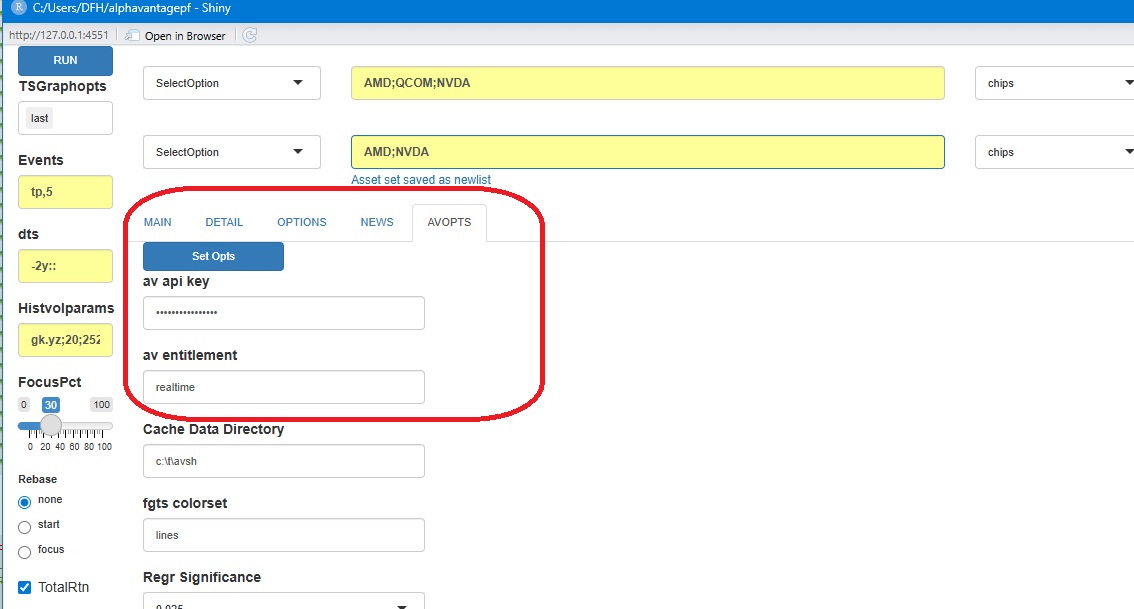
When the Set Opts button is pressed, a table of internal state variables is shown, with any changes highlighted. There are several options which can be set, all described in the Options Vignette, but one in particular is worth changing up front.

The app fills in a default data cache location determined by [tools::R_user_dir()]. Since that directory is a cache directory typically buried in long paths, you may find it helpful to set an alternative location in the Cache Data Directory field as has been done above. This will provide a consistent and easily accessable portal between the data used by the app and any external analyses or data collection mechanisms already in place.

After the first invocation, the app will start on the INVENTORY tab, so a user can immediately see what’s been updated and search for tickers.

General Usage

Analyses are all done by invoking “functions” or commands on a set of assets in the yellow line shown above. As described in the README file, commands which start with AV. are asset-less commands and mostly oriented towards app-specific information such as data inventories or help pages. All other commands refer to the semi-colon delimited asset or ticker list given first.

Once you know what you want, just type it in and hit “Enter”. The command will get any data it needs and then produce a set of tables, time series graphs, or other plots. See Data Vignette for details as to how this done. Most commands require a timeframe of historical data to analyze. The date range (formatted as above) in HistDates is used, but other date ranges within that range may be added as parameters.

The app responds as follows:

• Most results will appear in the MAIN tab, but some results may appear in function specific tabs. For example, the OPTIONS tab has specific fields to search for Equity options, and the NEWS tab has specific fields to narrow search results. Note that there is also a separate INVENTORY tab to always have a searchable ticker list available.

• By design, time series graphs are shown first, followed by tables and then ggplots. THe app allows for two independent time series graphs to be shown on top of each other. The second graph is typically made by adding a “2” onto the end of the command.

• Some commands may produce some auxiliary information in a separate tab. That tab is typically called DETAIL but can change names to highlight existence of results in the tab.

• Feedback (i.e.an error message) is placed below the command line, but can appear elsewhere. Progress messages will show in the R Console ²

Examples

You might want to start with AV.H which describes all the commands available. Some examples of commands that can be run are

Command	Description
EEM;HEEM GP	Graph raw time series of the EEM ETF and it’s hedged counterpart.
QQQ;SPY GPI2	Graph time series of QQQ and SPY rebased to 100 at start below the first graph.
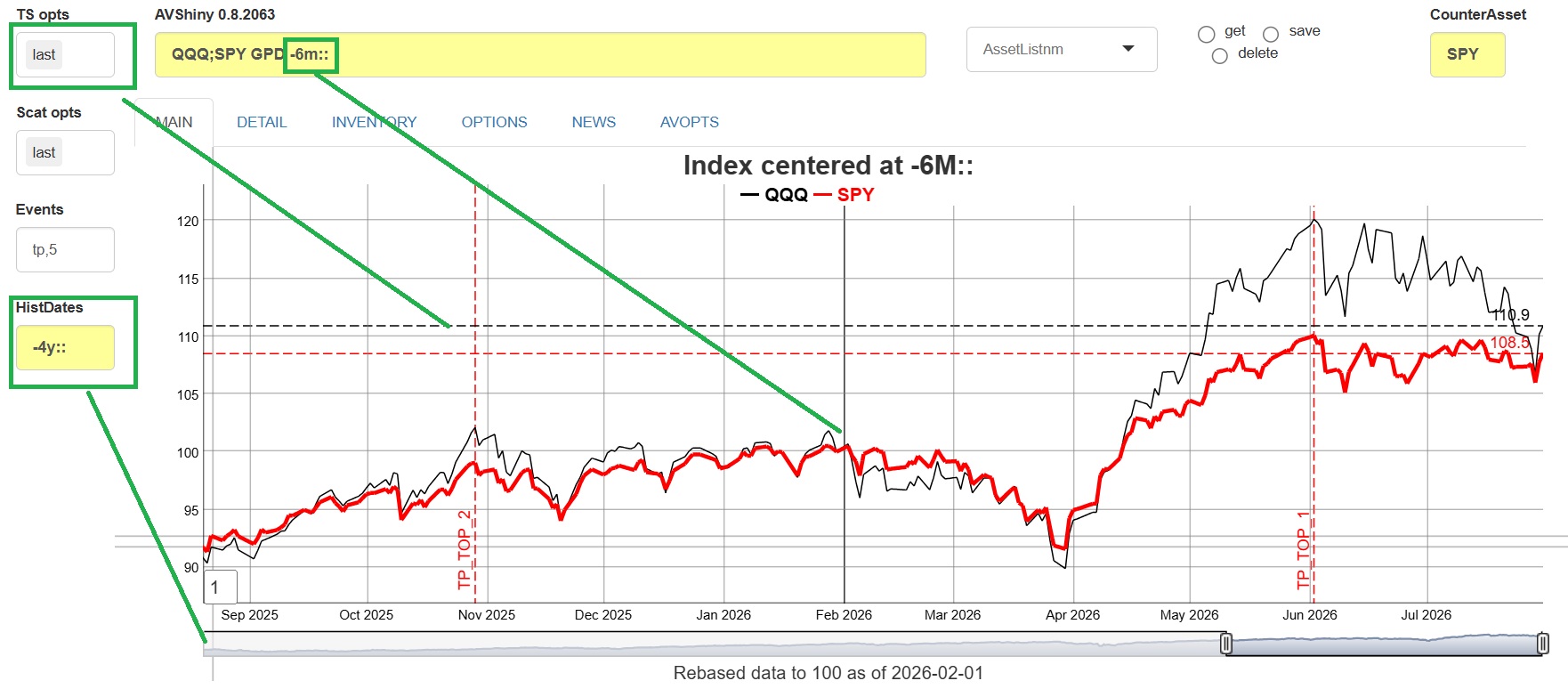
QQQ;SPY GPD -6m::	Graph total return indices of the two ETFs rebased to 100 as of 6 months ago
IBM;ORCL EA	Table of earnings and estimates for IBM and ORCL
IBM;ORCL GEP	Graph Earnings Yield for IBM and ORCL
IBM;ORCL CN	Table of linked News items for IBM and ORCL
IBM;ORCL DES	Table of descriptive items for IBM and ORCL
ORCL OS	Table of options for ORCL
ORCL RV	Active returns and correlations with the counterasset (default is SPY)
AV.EQINV	Show a list of all ETFs and Equities with downloaded data

To see how the date conventions work, the results of the third command are shown below. Note that there is a slider (provided by dygraphs()) which allows you to zoom in or out to specific time windows. In this case, the graph starts at -6m::, where both indices are rebased to 100, but can be zoomed out to a maximum of 4 years (HistDates has -4y::) from today. Finally, the last option in TSopts puts a horizontal bar showing the last values of each series.

gpd2 Example

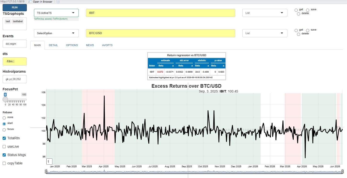
Here is another example which highlights both the comprehensive abilities to combine assets in the app with graphing abilities. Suppose we wish to plot the fair value history of the crypto ETF IBIT, and add some visual indication of overall market direction. Editing the counterasset to BTC/USD adding doi:regm in Events, and running IBIT RV gives the following.

Asset Lists

Securities are seldom analyzed in isolation. It is easy to create and use ad-hoc groups of securities in this app.

• To create a list, First, type in a new name for the list in the AssetListnm list box as shown below. Hit “enter” to add the name to the set of asset lists already in existence. (The Enter is necessary for Shiny to know that it’s a new identifier.) Then either type in the components into the Command line, or use the assets already in the asset line. Remenber lists are semi-colon delimited. Then hit the set button to save the list.

• To get the assets in a list, select the desired list from the dropdown and hit get button. The app will replace whatever assets you have in the command line with those from the desired list, leaving the command in place.

The best way to see how this works is with a short clip:

You can see a table of current asset lists by running the AV.INV command, and can add asset lists outside of the app using av_add_assetgroups(). See Data Vignette for details.

Specific command notes

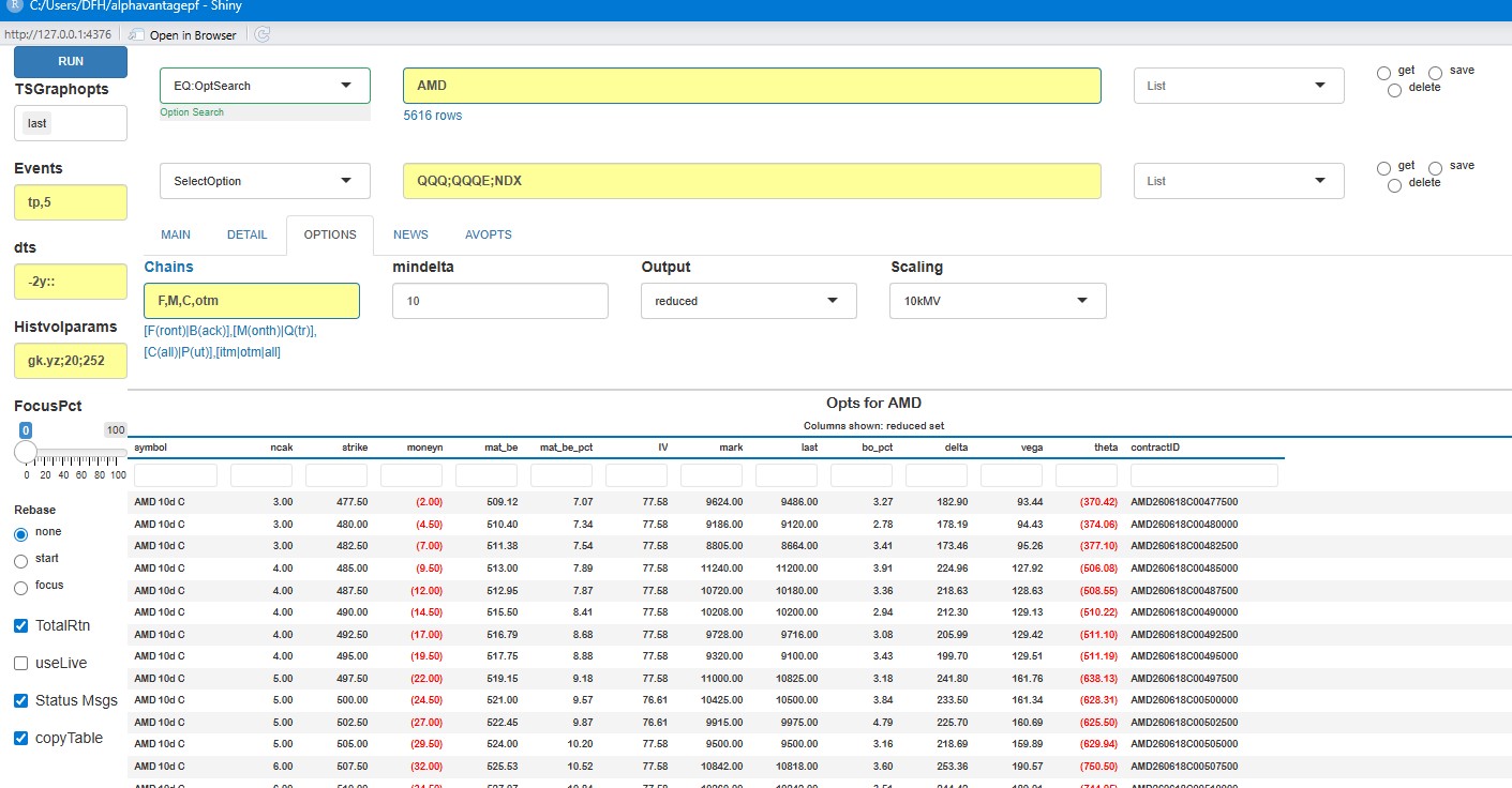
Options Search

To find options for a given set of tickers use the command OS, which will take you to the OPTIONS tab. A few fields on that page which will help narrow down the options are:

Field	Detail
Chains	Comma delimited string of four items to narrow downloaded options.
	1. [F|B] first contract or second contract
	2. [M|Q] Monthly expiration or Quarterly expiration
	3. [C|P|A] Calls, Puts or Both
	4. [itm|otm|all] In or out of the money3
Mindelta	Minimum absolute delta of option
Output	Subset of columns to show, relevant to Trading or Valuation
Scaling	Values and Greeks for 10 contracts or 10kUSD premium

The options change can be overridden as parameters to the OS call, as seen below. WIthout the parameters added on the command line, calls would have been returned.

[^1]: A “cheatsheet” with these conventions is displayed when AV.H is run, unless the showGeneralHelp option is deselected.